Learn you some Erlang

for great good!

• Home
• FAQ
• RSS
• Code

Recursion

Hello recursion!

Some readers accustomed with imperative and object-oriented programming languages might be wondering why loops weren't shown already. The answer to this is "what is a loop?" Truth is, functional programming languages usually do not offer looping constructs like for and while. Instead, functional programmers rely on a silly concept named recursion.

I suppose you remember how invariable variables were explained in the intro chapter. If you don't, you can give them more attention! Recursion can also be explained with the help of mathematical concepts and functions. A basic mathematical function such as the factorial of a value is a good example of a function that can be expressed recursively. The factorial of a number n is the product of the sequence 1 x 2 x 3 x ... x n, or alternatively n x (n-1) x (n-2) x ... x 1. To give some examples, the factorial of 3 is 3! = 3 x 2 x 1 = 6. The factorial of 4 would be 4! = 4 x 3 x 2 x 1 = 24. Such a function can be expressed the following way in mathematical notation:

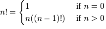
What this tells us is that if the value of n we have is 0, we return the result 1. For any value above 0, we return n multiplied by the factorial of n-1, which unfolds until it reaches 1:

4! = 4 x 3!
4! = 4 x 3 x 2!
4! = 4 x 3 x 2 x 1!
4! = 4 x 3 x 2 x 1 x 1

How can such a function be translated from mathematical notation to Erlang? The conversion is simple enough. Take a look at the parts of the notation: n!, 1 and n((n-1)!) and then the ifs. What we've got here is a function name (n!), guards (the ifs) and a the function body (1 and n((n-1)!)). We'll rename n! to fac(N) to restrict our syntax a bit and then we get the following:

-module(recursive).
-export([fac/1]).

fac(N) when N == 0 -> 1;
fac(N) when N > 0  -> N*fac(N-1).

And this factorial function is now done! It's pretty similar to the mathematical definition, really. With the help of pattern matching, we can shorten the definition a bit:

fac(0) -> 1;
fac(N) when N > 0 -> N*fac(N-1).

So that's quick and easy for some mathematical definitions which are recursive in nature. We looped! A definition of recursion could be made short by saying "a function that calls itself." However, we need to have a stopping condition (the real term is base case), because we'd otherwise loop infinitely. In our case, the stopping condition is when n is equal to 0. At that point we no longer tell our function to call itself and it stops its execution right there.

Length

Let's try to make it slightly more practical. We'll implement a function to count how many elements a list contains. So we know from the beginning that we will need:

• a base case;
• a function that calls itself;
• a list to try our function on.

With most recursive functions, I find the base case easier to write first: what's the simplest input we can have to find a length from? Surely an empty list is the simplest one, with a length of 0. So let's make a mental note that [] = 0 when dealing with lengths. Then the next simplest list has a length of 1: [_] = 1. This sounds like enough to get going with our definition. We can write this down:

len([]) -> 0;
len([_]) -> 1.

Awesome! We can calculate the length of lists, given the length is either 0 or 1! Very useful indeed. Well of course it's useless, because it's not yet recursive, which brings us to the hardest part: extending our function so it calls itself for lists longer than 1 or 0. It was mentioned earlier that lists are defined recursively as [1 | [2| ... [n | []]]]. This means we can use the [H|T] pattern to match against lists of one or more elements, as a list of length one will be defined as [X|[]] and a list of length two will be defined as [X|[Y|[]]]. Note that the second element is a list itself. This means we only need to count the first one and the function can call itself on the second element. Given each value in a list counts as a length of 1, the function can be rewritten the following way:

len([]) -> 0;
len([_|T]) -> 1 + len(T).

And now you've got your own recursive function to calculate the length of a list. To see how len/1 would behave when ran, let's try it on a given list, say [1,2,3,4]:

len([1,2,3,4]) = len([1 | [2,3,4])
               = 1 + len([2 | [3,4]])
               = 1 + 1 + len([3 | [4]])
               = 1 + 1 + 1 + len([4 | []])
               = 1 + 1 + 1 + 1 + len([])
               = 1 + 1 + 1 + 1 + 0
               = 1 + 1 + 1 + 1
               = 1 + 1 + 2
               = 1 + 3 
               = 4

Which is the right answer. Congratulations on your first useful recursive function in Erlang!

Length of a Tail Recursion

You might have noticed that for a list of 4 terms, we expanded our function call to a single chain of 5 additions. While this does the job fine for short lists, it can become problematic if your list has a few million values in it. You don't want to keep millions of numbers in memory for such a simple calculation. It's wasteful and there's a better way. Enter tail recursion.

Tail recursion is a way to transform the above linear process (it grows as much as there are elements) to an iterative one (there is not really any growth). To have a function call being tail recursive, it needs to be 'alone'. Let me explain: what made our previous calls grow is how the answer of the first part depended on evaluating the second part. The answer to 1 + len(Rest) needs the answer of len(Rest) to be found. The function len(Rest) itself then needed the result of another function call to be found. The additions would get stacked until the last one is found, and only then would the final result be calculated. Tail recursion aims to eliminate this stacking of operation by reducing them as they happen.

In order to achieve this, we will need to hold an extra temporary variable as a parameter in our function. I'll illustrate the concept with the help of the factorial function, but this time defining it to be tail recursive. The aforementioned temporary variable is sometimes called accumulator and acts as a place to store the results of our computations as they happen in order to limit the growth of our calls:

tail_fac(N) -> tail_fac(N,1).

tail_fac(0,Acc) -> Acc;
tail_fac(N,Acc) when N > 0 -> tail_fac(N-1,N*Acc).

Here, I define both tail_fac/1 and tail_fac/2. The reason for this is that Erlang doesn't allow default arguments in functions (different arity means different function) so we do that manually. In this specific case, tail_fac/1 acts like an abstraction over the tail recursive tail_fac/2 function. The details about the hidden accumulator of tail_fac/2 don't interest anyone, so we would only export tail_fac/1 from our module. When running this function, we can expand it to:

tail_fac(4)    = tail_fac(4,1)
tail_fac(4,1)  = tail_fac(4-1, 4*1)
tail_fac(3,4)  = tail_fac(3-1, 3*4)
tail_fac(2,12) = tail_fac(2-1, 2*12)
tail_fac(1,24) = tail_fac(1-1, 1*24)
tail_fac(0,24) = 24

See the difference? Now we never need to hold more than two terms in memory: the space usage is constant. It will take as much space to calculate the factorial of 4 as it will take space to calculate the factorial of 1 million (if we forget 4! is a smaller number than 1M! in its complete representation, that is).

With an example of tail recursive factorials under your belt, you might be able to see how this pattern could be applied to our len/1 function. What we need is to make our recursive call 'alone'. If you like visual examples, just imagine you're going to put the +1 part inside the function call by adding a parameter:

len([]) -> 0;
len([_|T]) -> 1 + len(T).

becomes:

tail_len(L) -> tail_len(L,0).

tail_len([], Acc) -> Acc;
tail_len([_|T], Acc) -> tail_len(T,Acc+1).

And now your length function is tail recursive.

More recursive functions

We'll write a few more recursive functions, just to get in the habit a bit more. After all, recursion being the only looping construct that exists in Erlang (except list comprehensions), it's one of the most important concepts to understand. It's also useful in every other functional programming language you'll try afterwards, so take notes!

The first function we'll write will be duplicate/2. This function takes an integer as its first parameter and then any other term as its second parameter. It will then create a list of as many copies of the term as specified by the integer. Like before, thinking of the base case first is what might help you get going. For duplicate/2, asking to repeat something 0 time is the most basic thing that can be done. All we have to do is return an empty list, no matter what the term is. Every other case needs to try and get to the base case by calling the function itself. We will also forbid negative values for the integer, because you can't duplicate something -n times:

duplicate(0,_) ->
    [];
duplicate(N,Term) when N > 0 ->
    [Term|duplicate(N-1,Term)].

Once the basic recursive function is found, it becomes easier to transform it into a tail recursive one by moving the list construction into a temporary variable:

tail_duplicate(N,Term) ->
    tail_duplicate(N,Term,[]).

tail_duplicate(0,_,List) ->
    List;
tail_duplicate(N,Term,List) when N > 0 ->
    tail_duplicate(N-1, Term, [Term|List]).

Success! I want to change the subject a little bit here by drawing a parallel between tail recursion and a while loop. Our tail_duplicate/2 function has all the usual parts of a while loop. If we were to imagine a while loop in a fictional language with Erlang-like syntax, our function could look a bit like this:

function(N, Term) ->
    while N > 0 ->
        List = [Term|List],
        N = N-1
    end,
    List.

Note that all the elements are there in both the fictional language and in Erlang. Only their position changes. This demonstrates that a proper tail recursive function is similar to an iterative process, like a while loop.

There's also an interesting property that we can 'discover' when we compare recursive and tail recursive functions by writing a reverse/1 function, which will reverse a list of terms. For such a function, the base case is an empty list, for which we have nothing to reverse. We can just return an empty list when that happens. Every other possibility should try to converge to the base case by calling itself, like with duplicate/2. Our function is going to iterate through the list by pattern matching [H|T] and then putting H after the rest of the list:

reverse([]) -> [];
reverse([H|T]) -> reverse(T)++[H].

On long lists, this will be a true nightmare: not only will we stack up all our append operations, but we will need to traverse the whole list for every single of these appends until the last one! For visual readers, the many checks can be represented as:

reverse([1,2,3,4]) = [4]++[3]++[2]++[1]
                      ↑    ↵
                   = [4,3]++[2]++[1]
                      ↑ ↑    ↵
                   = [4,3,2]++[1]
                      ↑ ↑ ↑    ↵
                   = [4,3,2,1]

This is where tail recursion comes to the rescue. Because we will use an accumulator and will add a new head to it every time, our list will automatically be reversed. Let's first see the implementation:

tail_reverse(L) -> tail_reverse(L,[]).

tail_reverse([],Acc) -> Acc;
tail_reverse([H|T],Acc) -> tail_reverse(T, [H|Acc]).

If we represent this one in a similar manner as the normal version, we get:

tail_reverse([1,2,3,4]) = tail_reverse([2,3,4], [1])
                        = tail_reverse([3,4], [2,1])
                        = tail_reverse([4], [3,2,1])
                        = tail_reverse([], [4,3,2,1])
                        = [4,3,2,1]   

Which shows that the number of elements visited to reverse our list is now linear: not only do we avoid growing the stack, we also do our operations in a much more efficient manner!

Another function to implement could be sublist/2, which takes a list L and an integer N, and returns the N first elements of the list. As an example, sublist([1,2,3,4,5,6],3) would return [1,2,3]. Again, the base case is trying to obtain 0 elements from a list. Take care however, because sublist/2 is a bit different. You've got a second base case when the list passed is empty! If we do not check for empty lists, an error would be thrown when calling recursive:sublist([1],2). while we want [1] instead. Once this is defined, the recursive part of the function only has to cycle through the list, keeping elements as it goes, until it hits one of the base cases:

sublist(_,0) -> [];
sublist([],_) -> [];
sublist([H|T],N) when N > 0 -> [H|sublist(T,N-1)].

Which can then be transformed to a tail recursive form in the same manner as before:

tail_sublist(L, N) -> tail_sublist(L, N, []).

tail_sublist(_, 0, SubList) -> SubList;
tail_sublist([], _, SubList) -> SubList;
tail_sublist([H|T], N, SubList) when N > 0 ->
    tail_sublist(T, N-1, [H|SubList]).

There's a flaw in this function. A fatal flaw! We use a list as an accumulator in exactly the same manner we did to reverse our list. If you compile this function as is, sublist([1,2,3,4,5,6],3) would not return [1,2,3], but [3,2,1]. The only thing we can do is take the final result and reverse it ourselves. Just change the tail_sublist/2 call and leave all our recursive logic intact:

tail_sublist(L, N) -> reverse(tail_sublist(L, N, [])).

The final result will be ordered correctly. It might seem like reversing our list after a tail recursive call is a waste of time and you would be partially right (we still save memory doing this). On shorter lists, you might find your code is running faster with normal recursive calls than with tail recursive calls for this reason, but as your data sets grow, reversing the list will be comparatively lighter.

To push things a bit further, we'll write a zipping function. A zipping function will take two lists of same length as parameters and will join them as a list of tuples which all hold two terms. Our own zip/2 function will behave this way:

1> recursive:zip([a,b,c],[1,2,3]).
[{a,1},{b,2},{c,3}]

Given we want our parameters to both have the same length, the base case will be zipping two empty lists:

zip([],[]) -> [];
zip([X|Xs],[Y|Ys]) -> [{X,Y}|zip(Xs,Ys)].

However, if you wanted a more lenient zip function, you could decide to have it finish whenever one of the two list is done. In this scenario, you therefore have two base cases:

lenient_zip([],_) -> [];
lenient_zip(_,[]) -> [];
lenient_zip([X|Xs],[Y|Ys]) -> [{X,Y}|lenient_zip(Xs,Ys)].

Notice that no matter what our base cases are, the recursive part of the function remains the same. I would suggest you try and make your own tail recursive versions of zip/2 and lenient_zip/2, just to make sure you fully understand how to make tail recursive functions: they'll be one of the central concepts of larger applications where our main loops will be made that way.

If you want to check your answers, take a look at my implementation of recursive.erl, more precisely the tail_zip/2 and tail_lenient_zip/3 functions.

Quick, Sort!

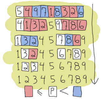
I can (and will) now assume recursion and tail recursion make sense to you, but just to make sure, I'm going to push for a more complex example, quicksort. Yes, the traditional "hey look I can write short functional code" canonical example. A naive implementation of quicksort works by taking the first element of a list, the pivot, and then putting all the elements smaller or equal to the pivot in a new list, and all those larger in another list. We then take each of these lists and do the same thing on them until each list gets smaller and smaller. This goes on until you have nothing but an empty list to sort, which will be our base case. This implementation is said to be naive because smarter versions of quicksort will try to pick optimal pivots to be faster. We don't really care about that for our example though.

We will need two functions for this one: a first function to partition the list into smaller and larger parts and a second function to apply the partition function on each of the new lists and to glue them together. First of all, we'll write the glue function:

quicksort([]) -> [];
quicksort([Pivot|Rest]) ->
    {Smaller, Larger} = partition(Pivot,Rest,[],[]),
    quicksort(Smaller) ++ [Pivot] ++ quicksort(Larger).

This shows the base case, a list already partitioned in larger and smaller parts by another function, the use of a pivot with both lists quicksorted appended before and after it. So this should take care of assembling lists. Now the partitioning function:

partition(_,[], Smaller, Larger) -> {Smaller, Larger};
partition(Pivot, [H|T], Smaller, Larger) ->
    if H =< Pivot -> partition(Pivot, T, [H|Smaller], Larger);
       H >  Pivot -> partition(Pivot, T, Smaller, [H|Larger])
    end. 

And you can now run your quicksort function. If you've looked for Erlang examples on the Internet before, you might have seen another implementation of quicksort, one that is simpler and easier to read, but makes use of list comprehensions. The easy to replace parts are the ones that create new lists, the partition/4 function:

lc_quicksort([]) -> [];
lc_quicksort([Pivot|Rest]) ->
    lc_quicksort([Smaller || Smaller <- Rest, Smaller =< Pivot])
    ++ [Pivot] ++
    lc_quicksort([Larger || Larger <- Rest, Larger > Pivot]).

The main differences are that this version is much easier to read, but in exchange, it has to traverse the list twice to partition it in two parts. This is a fight of clarity against performance, but the real loser here is you, because a function lists:sort/1 already exists. Use that one instead.

More than lists

By reading this chapter, you might be starting to think recursion in Erlang is mainly a thing concerning lists. While lists are a good example of a data structure that can be defined recursively, there's certainly more than that. For the sake of diversity, we'll see how to build binary trees, and then read data from them.

First of all, it's important to define what a tree is. In our case, it's nodes all the way down. Nodes are tuples that contain a key, a value associated to the key, and then two other nodes. Of these two nodes, we need one that has a smaller and one that has a larger key than the node holding them. So here's recursion! A tree is a node containing nodes, each of which contains nodes, which in turn also contain nodes. This can't keep going forever (we don't have infinite data to store), so we'll say that our nodes can also contain empty nodes.

To represent nodes, tuples are an appropriate data structure. For our implementation, we can then define these tuples as {node, {Key, Value, Smaller, Larger}} (a tagged tuple!), where Smaller and Larger can be another similar node or an empty node ({node, nil}). We won't actually need a concept more complex than that.

Let's start building a module for our very basic tree implementation. The first function, empty/0, returns an empty node. The empty node is the starting point of a new tree, also called the root:

-module(tree).
-export([empty/0, insert/3, lookup/2]).

empty() -> {node, 'nil'}.

By using that function and then encapsulating all representations of nodes the same way, we hide the implementation of the tree so people don't need to know how it's built. All that information can be contained by the module alone. If you ever decide to change the representation of a node, you can then do it without breaking external code.

To add content to a tree, we must first understand how to recursively navigate through it. Let's proceed in the same way as we did for every other recursion example by trying to find the base case. Given that an empty tree is an empty node, our base case is thus logically an empty node. So whenever we'll hit an empty node, that's where we can add our new key/value. The rest of the time, our code has to go through the tree trying to find an empty node where to put content.

To find an empty node starting from the root, we must use the fact that the presence of Smaller and Larger nodes let us navigate by comparing the new key we have to insert to the current node's key. If the new key is smaller than the current node's key, we try to find the empty node inside Smaller, and if it's larger, inside Larger. There is one last case, though: what if the new key is equal to the current node's key? We have two options there: let the program fail or replace the value with the new one. This is the option we'll take here. Put into a function all this logic works the following way:

insert(Key, Val, {node, 'nil'}) ->
    {node, {Key, Val, {node, 'nil'}, {node, 'nil'}}};
insert(NewKey, NewVal, {node, {Key, Val, Smaller, Larger}}) when NewKey < Key ->
    {node, {Key, Val, insert(NewKey, NewVal, Smaller), Larger}};
insert(NewKey, NewVal, {node, {Key, Val, Smaller, Larger}}) when NewKey > Key ->
    {node, {Key, Val, Smaller, insert(NewKey, NewVal, Larger)}};
insert(Key, Val, {node, {Key, _, Smaller, Larger}}) ->
    {node, {Key, Val, Smaller, Larger}}.

Note here that the function returns a completely new tree. This is typical of functional languages having only single assignment. While this can be seen as inefficient, most of the underlying structures of two versions of a tree sometimes happen to be the same and are thus shared, copied by the VM only when needed.

What's left to do on this example tree implementation is creating a lookup/2 function that will let you find a value from a tree by giving its key. The logic needed is extremely similar to the one used to add new content to the tree: we step through the nodes, checking if the lookup key is equal, smaller or larger than the current node's key. We have two base cases: one when the node is empty (the key isn't in the tree) and one when the key is found. Because we don't want our program to crash each time we look for a key that doesn't exist, we'll return the atom 'undefined'. Otherwise, we'll return {ok, Value}. The reason for this is that if we only returned Value and the node contained the atom 'undefined', we would have no way to know if the tree did return the right value or failed to find it. By wrapping successful cases in such a tuple, we make it easy to understand which is which. Here's the implemented function:

lookup(_, {node, 'nil'}) ->
    undefined;
lookup(Key, {node, {Key, Val, _, _}}) ->
    {ok, Val};
lookup(Key, {node, {NodeKey, _, Smaller, _}}) when Key < NodeKey ->
    lookup(Key, Smaller);
lookup(Key, {node, {_, _, _, Larger}}) ->
    lookup(Key, Larger).

And we're done. Let's test it with by making a little email address book. Compile the file and start the shell:

1> T1 = tree:insert("Jim Woodland", "jim.woodland@gmail.com", tree:empty()).
{node,{"Jim Woodland","jim.woodland@gmail.com",
       {node,nil},
       {node,nil}}}
2> T2 = tree:insert("Mark Anderson", "i.am.a@hotmail.com", T1).
{node,{"Jim Woodland","jim.woodland@gmail.com",
       {node,nil},
       {node,{"Mark Anderson","i.am.a@hotmail.com",
              {node,nil},
              {node,nil}}}}}
3> Addresses = tree:insert("Anita Bath", "abath@someuni.edu", tree:insert("Kevin Robert", "myfairy@yahoo.com", tree:insert("Wilson Longbrow", "longwil@gmail.com", T2))).
{node,{"Jim Woodland","jim.woodland@gmail.com",
       {node,{"Anita Bath","abath@someuni.edu",
              {node,nil},
              {node,nil}}},
       {node,{"Mark Anderson","i.am.a@hotmail.com",
              {node,{"Kevin Robert","myfairy@yahoo.com",
                     {node,nil},
                     {node,nil}}},
              {node,{"Wilson Longbrow","longwil@gmail.com",
                     {node,nil},
                     {node,nil}}}}}}}

And now you can lookup email addresses with it:

4> tree:lookup("Anita Bath", Addresses).
{ok, "abath@someuni.edu"}
5> tree:lookup("Jacques Requin", Addresses).
undefined

That concludes our functional address book example built from a recursive data structure other than a list! Anita Bath now...

Thinking recursively

If you've understood everything in this chapter, thinking recursively is probably becoming more intuitive. A different aspect of recursive definitions when compared to their imperative counterparts (usually in while or for loops) is that instead of taking a step-by-step approach ("do this, then that, then this, then you're done"), our approach is more declarative ("if you get this input, do that, this otherwise"). This property is made more obvious with the help of pattern matching in function heads.

If you still haven't grasped how recursion works, maybe reading this will help you.

Joking aside, recursion coupled with pattern matching is sometimes an optimal solution to the problem of writing concise algorithms that are easy to understand. By subdividing each part of a problem into separate functions until they can no longer be simplified, the algorithm becomes nothing but assembling a bunch of correct answers coming from short routines (that's a bit similar to what we did with quicksort). This kind of mental abstraction is also possible with your everyday loops, but I believe the practice is easier with recursion. Your mileage may vary.

And now ladies and gentlemen, a discussion: the author vs. himself

• — Okay, I think I understand recursion. I get the declarative aspect of it. I get it has mathematical roots, like with invariable variables. I get that you find it easier in some cases. What else?
• — It respects a regular pattern. Find the base cases, write them down, then every other cases should try to converge to these base cases to get your answer. It makes writing functions pretty easy.
• — Yeah, I got that, you repeated it a bunch of times already. My loops can do the same.
• — Yes they can. Can't deny that!
• — Right. A thing I don't get is why you bothered writing all these non-tail recursive versions if they're not as good as tail recursive ones.
• — Oh it's simply to make things easier to grasp. Moving from regular recursion, which is prettier and easier to understand, to tail recursion, which is theoretically more efficient, sounded like a good way to show all options.
• — Right, so they're useless except for educational purposes, I get it.
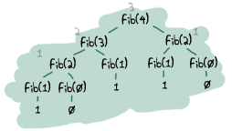
• — Not exactly. In practice you'll see little difference in the performance between tail recursive and normal recursive calls. The areas to take care of are in functions that are supposed to loop infinitely, like main loops. There's also a type of functions that will always generate very large stacks, be slow and possibly crash early if you don't make them tail recursive. The best example of this is the Fibonacci function, which grows exponentially if it's not iterative or tail recursive. You should profile your code (I'll show how to do that at a later point, I promise), see what slows it down, and fix it.
• — But loops are always iterative and make this a non-issue.
• — Yes, but... but... my beautiful Erlang...
• — Well isn't that great? All that learning because there is no 'while' or 'for' in Erlang. Thank you very much I'm going back to programming my toaster in C!
• — Not so fast there! Functional programming languages have other assets! If we've found some base case patterns to make our life easier when writing recursive functions, a bunch of smart people have found many more to the point where you will need to write very few recursive functions yourself. If you stay around, I'll show you how such abstractions can be built. But for this we will need more power. Let me tell you about higher order functions...

• < Previous
• Index
• Next >

Except where otherwise noted, content on this site is licensed under a Creative Commons Attribution Non-Commercial No Derivative License